Gradient Evolution | David Weissteiner

In this article, we investigate the behavior of gradients during training.

We consider several datasets that are highly popular in deep learning, and face both regression and classification tasks. For each of these datasets, we train a deep learning model and obtain the respective gradients during training, which we then analyze. All of these steps are implemented in Python using Tensorflow Keras.

If you are not interested in the code but only in the evaluations and results, we recommend to skip to the last chapter.

Setup

Library Imports

from enum import Enum
import matplotlib.animation as animplt
import matplotlib.pyplot as plt
import numpy as np
import os
import pandas as pd
from pathlib import Path
import pickle
from sklearn.preprocessing import LabelEncoder
import tensorflow as tf

Besides the library imports, we also define a seed for reproducibility.

seed = 13

Datasets

For performing the experiments, we take into consideration the following datasets:

For the sake of conciseness, we only include the implementations for Mnist in this article. Anyhow, we include the results of all datasets. The implementation for all datasets is accessible on GitHub.

Data Loading

For every dataset, we create a function to load the data as a tensorflow dataset. More specifically, each of these functions returns three datasets following the training-validation-test split. An instance in such a dataset comprises the explanatory features together with their respective response. Example Mnist:

def getMnistDataset():
    num_classes = 10

    (x_train, y_train), (x_test, y_test) = tf.keras.datasets.mnist.load_data()

    # scale the image values to [0, 1]
    x_train = x_train.astype("float32") / 255
    x_test = x_test.astype("float32") / 255

    # expand the image dimensions from (28, 28) to (28, 28, 1)
    x_train = np.expand_dims(x_train, -1)
    x_test = np.expand_dims(x_test, -1)

    # one-hot encode the labels
    y_train = tf.keras.utils.to_categorical(y_train, num_classes)
    y_test = tf.keras.utils.to_categorical(y_test, num_classes)

    # concatenate images with labels
    train = tf.data.Dataset.from_tensor_slices((x_train, y_train))
    test = tf.data.Dataset.from_tensor_slices((x_test, y_test))

    # split train dataset into train and validation set
    train, val = tf.keras.utils.split_dataset(train, left_size=0.9, right_size=None,
        shuffle=True, seed=seed)

    return train, val, test

Finally, we obtain our desired dataset by invoking this function.

train, val, test = getMnistDataset()

Building the Model

Since each of the datasets is different, we have to build individual deep learning models depending on the dataset choice. Therefore, we define a function for every dataset which builds and compiles the corresponding model. Example Mnist:

def getMnistModel(data_element_spec):
    num_classes = data_element_spec[1].shape[0]

    keras_model = tf.keras.Sequential()
    keras_model.add(tf.keras.Input(shape=data_element_spec[0].shape))

    keras_model.add(tf.keras.layers.Conv2D(32, kernel_size=(3, 3), activation="relu",
        kernel_initializer=tf.keras.initializers.GlorotUniform(seed=seed),
        bias_initializer=tf.keras.initializers.Zeros()))
    keras_model.add(tf.keras.layers.MaxPool2D(pool_size=(2, 2)))
    keras_model.add(tf.keras.layers.Conv2D(64, kernel_size=(3, 3), activation="relu",
        kernel_initializer=tf.keras.initializers.GlorotUniform(seed=seed),
        bias_initializer=tf.keras.initializers.Zeros()))
    keras_model.add(tf.keras.layers.MaxPool2D(pool_size=(2, 2)))
    keras_model.add(tf.keras.layers.Flatten())
    keras_model.add(tf.keras.layers.Dropout(0.5, seed=seed))
    keras_model.add(tf.keras.layers.Dense(num_classes, activation="softmax",
        kernel_initializer=tf.keras.initializers.GlorotUniform(seed=seed),
        bias_initializer=tf.keras.initializers.Zeros()))

    optimizer = tf.keras.optimizers.SGD(
        learning_rate=0.01)
    keras_model.compile(optimizer=optimizer,
        loss=tf.keras.losses.CategoricalCrossentropy(),
        metrics=[tf.metrics.CategoricalCrossentropy(),
            tf.metrics.CategoricalAccuracy()])

    return keras_model

Just like before, we invoke this function to obtain our model.

model = getMnistModel(train.element_spec)

Fitting the Model

When fitting the model, we compute the gradient for every data batch individually and apply it to the model parameters. Thereby, we collect not only the overall gradient for an entire epoch but also the gradient for every minibatch step.

To do so, we create a function to perform a single epoch of training which yields the overall (i.e., accumulated) gradient, the individual gradients from the minibatch steps, and some evaluation metrics.

def fitGradient(model, train, loss_obj):
    train_metrics = None
    individual_gradients = list()

    for step, (x_batch_train, y_batch_train) in enumerate(train):
        with tf.GradientTape() as tape:
            preds = model(x_batch_train, training=True)
            loss_value = loss_obj()(y_batch_train, preds)
        grad = tape.gradient(loss_value, model.trainable_variables)
        model.optimizer.apply_gradients(zip(grad, model.trainable_variables))
        grad = np.array([g.numpy() for g in grad], dtype=object)
        individual_gradients.append(grad)
        if(step == 0):
            accumulated_grad = grad.copy()
        else:
            accumulated_grad += grad

    evaluation_scalars = model.evaluate(train, verbose=2)
    scalar_train_metrics = dict(zip(model.metrics_names, evaluation_scalars))
    if(train_metrics == None):
        train_metrics = {mname: [mval] for mname, mval in scalar_train_metrics.items()}
    else:
        for mname, mval in scalar_train_metrics.items():
            train_metrics[mname].append(mval)

    return accumulated_grad, train_metrics, individual_gradients

Utilizing this function, we then perform model training for the desired number of epochs in a loop while collecting the resulting gradients and metrics.

BATCH_SIZE = 256
NUM_EPOCHS = 10
LOSS = tf.keras.losses.CategoricalCrossentropy

gradients = list()
metrics = list()
individual_gradients = list()

for epoch in range(NUM_EPOCHS):
    grad, metr, ind_grad = fitGradient(model, train.batch(batch_size=BATCH_SIZE), LOSS)

    gradients.append(grad)
    metrics.append(metr)
    individual_gradients.extend(ind_grad)

Statistics and Plotting

After the collection of all gradients and metrics during training, we can use them to investigate the behavior of the gradient.

Statistics

As we are mostly interested in the magnitude of the gradient during the fitting process, we consider the L1 vector norm of our gradient as a metric for its magnitude. However, since we cannot directly compute the vector norm of a gradient, we first flatten the gradient layers and then sum up their vector norms. That way, we compute the vector norm of all gradients.

statistics = dict()
statistics["l1_norm_standardized"] = [np.sum([np.linalg.norm(layer_grad.flatten(), ord=1) / layer_grad.size
    for layer_grad in grad]) for grad in gradients]

In addition, we consider the accumulation of all gradients (i.e., the cumulative sum of gradients) to understand their eventual impact on the model parameters better. Therefore, we first compute the cumulative sum of the gradients followed by the vector norm in the same way as before.

accumulated_gradients = np.cumsum(gradients, axis=0)
statistics["l1_norm_acc_standardized"] = [np.sum([np.linalg.norm(layer_grad.flatten(), ord=1) / layer_grad.size
    for layer_grad in accgrad]) for accgrad in accumulated_gradients]

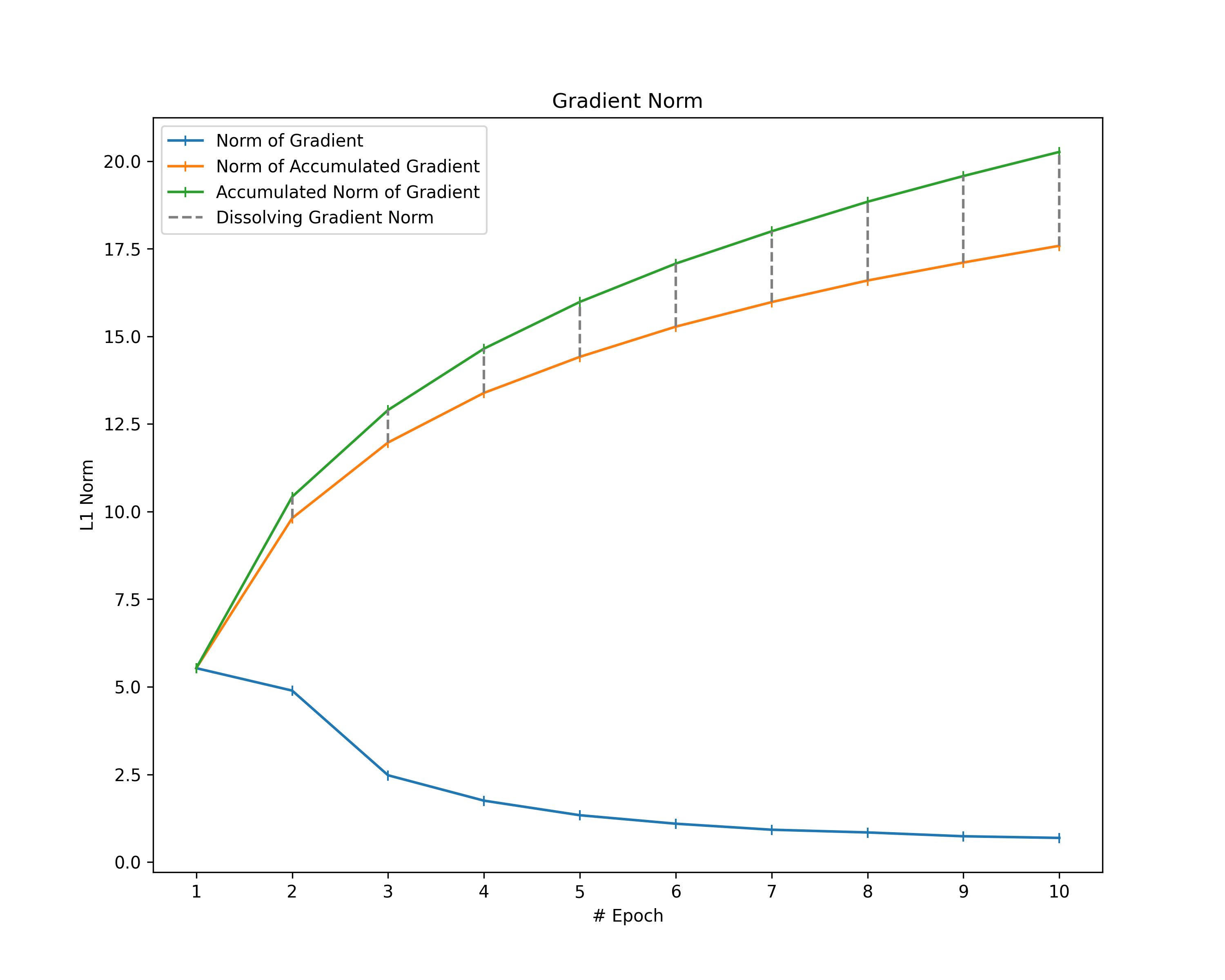
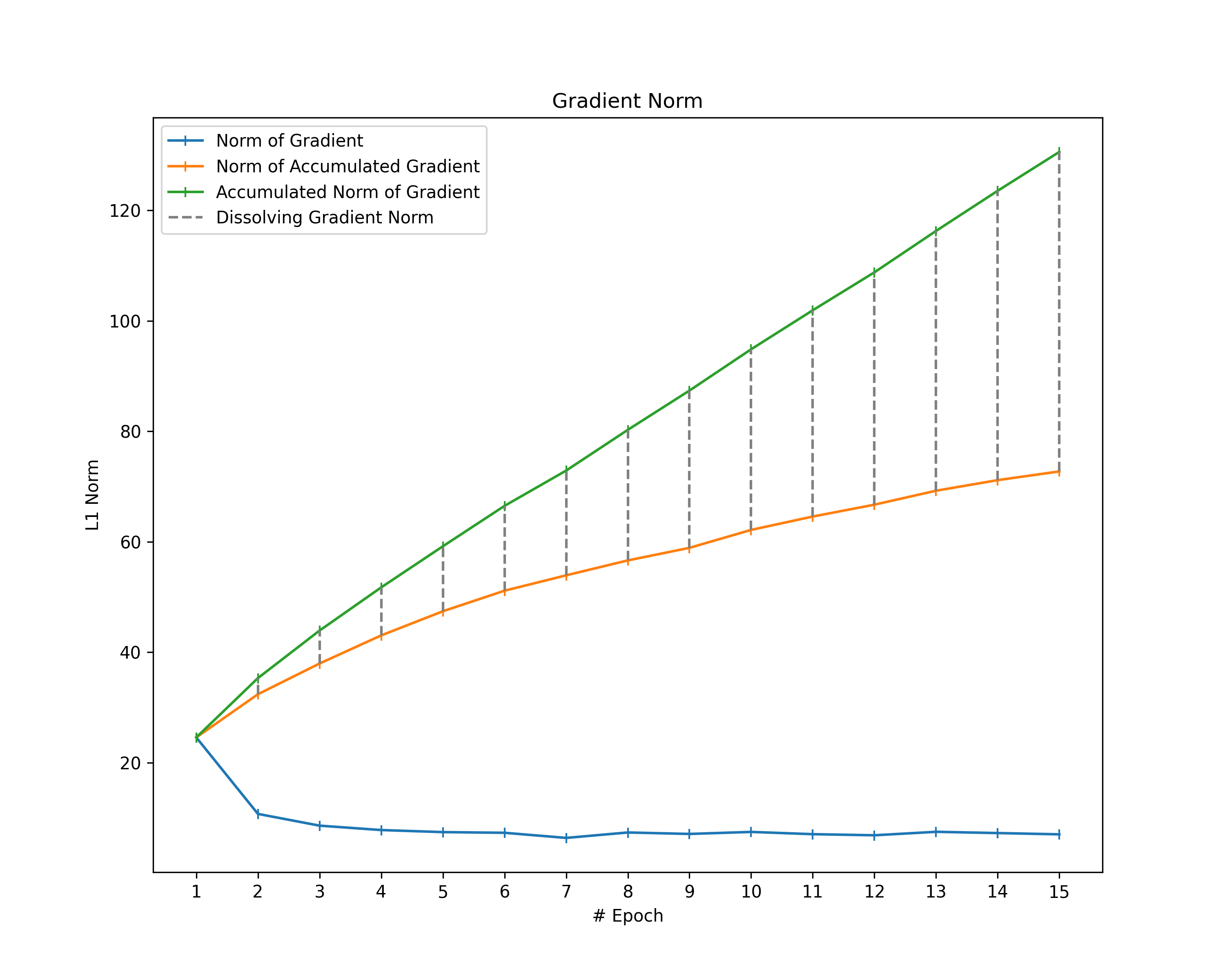
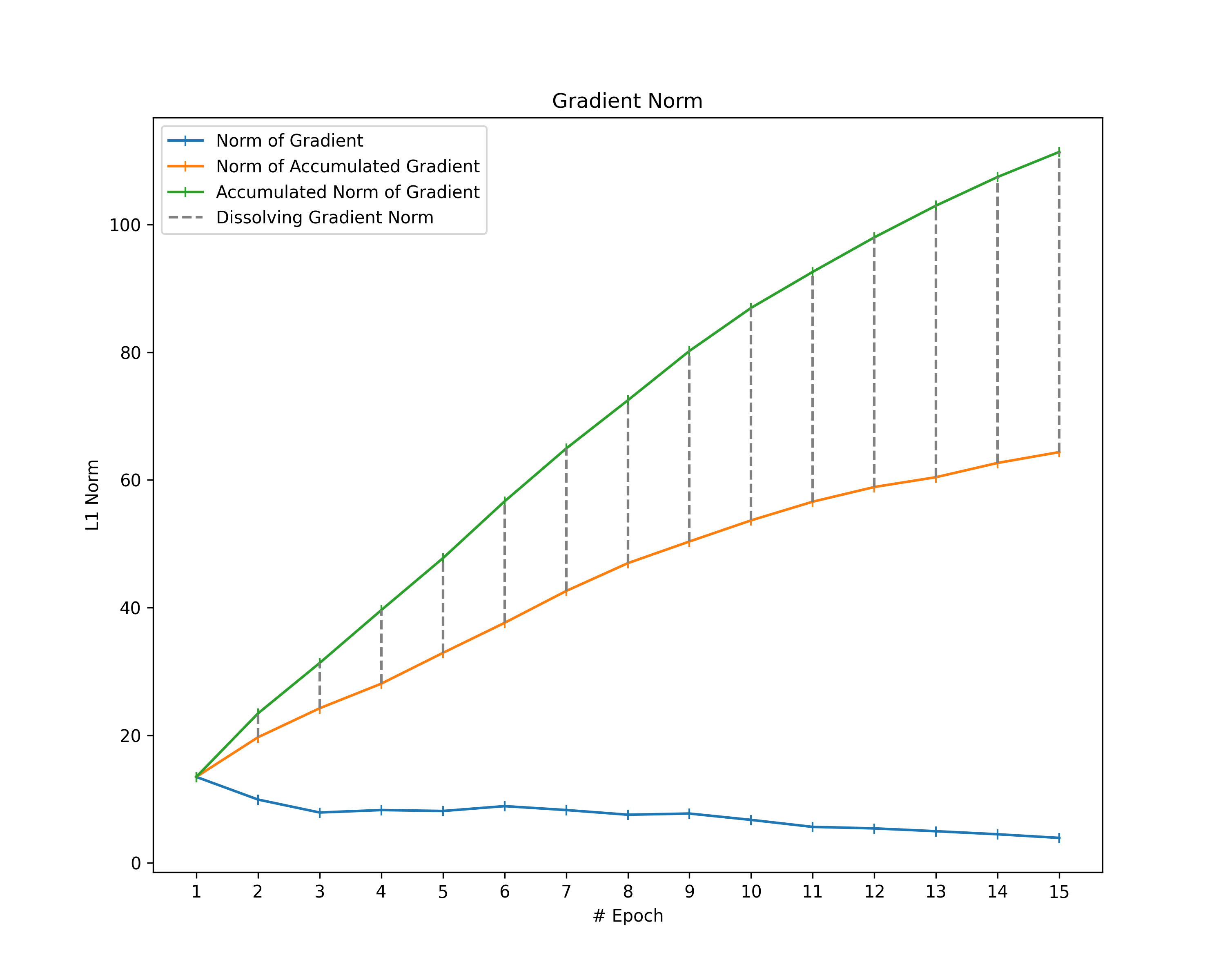
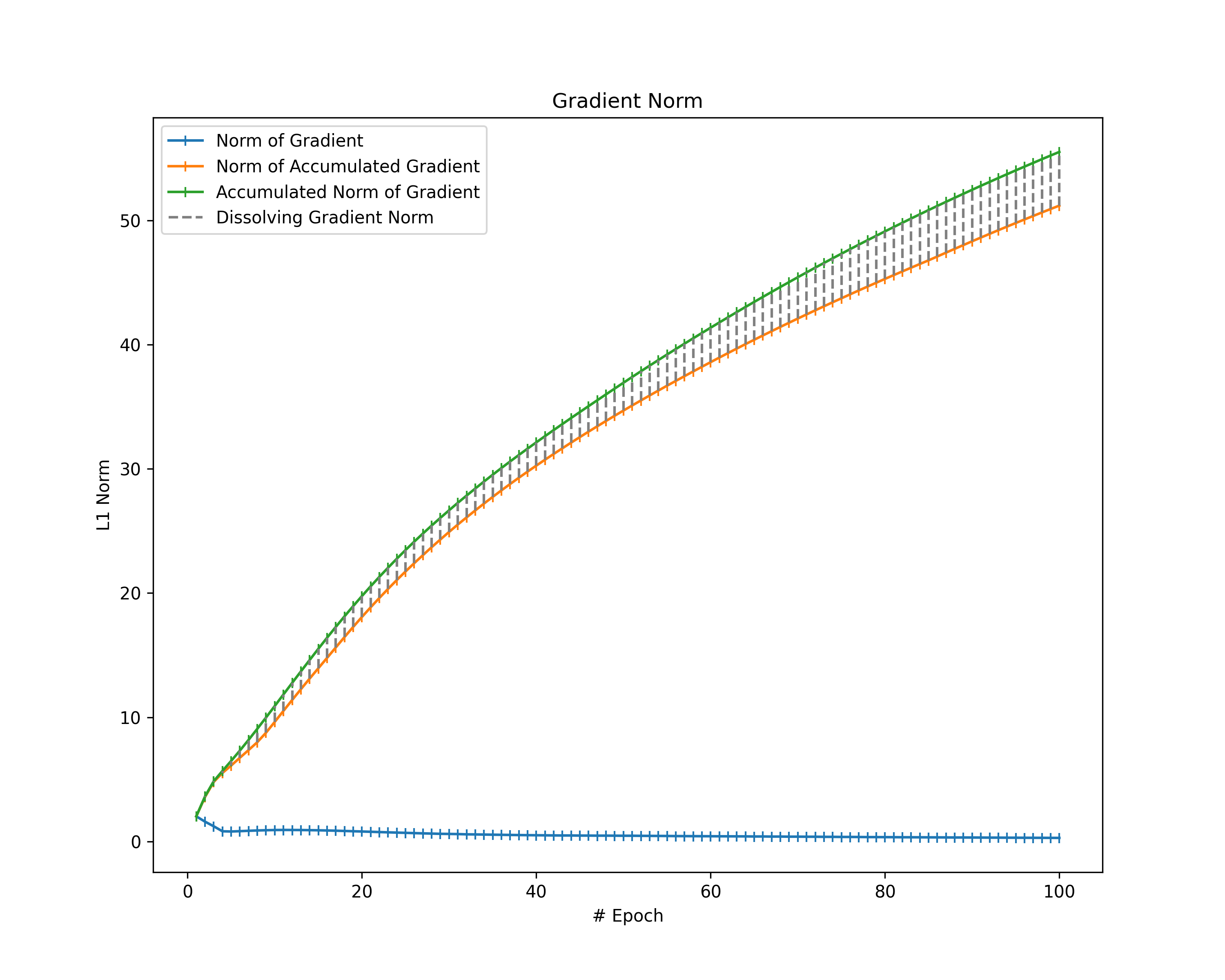
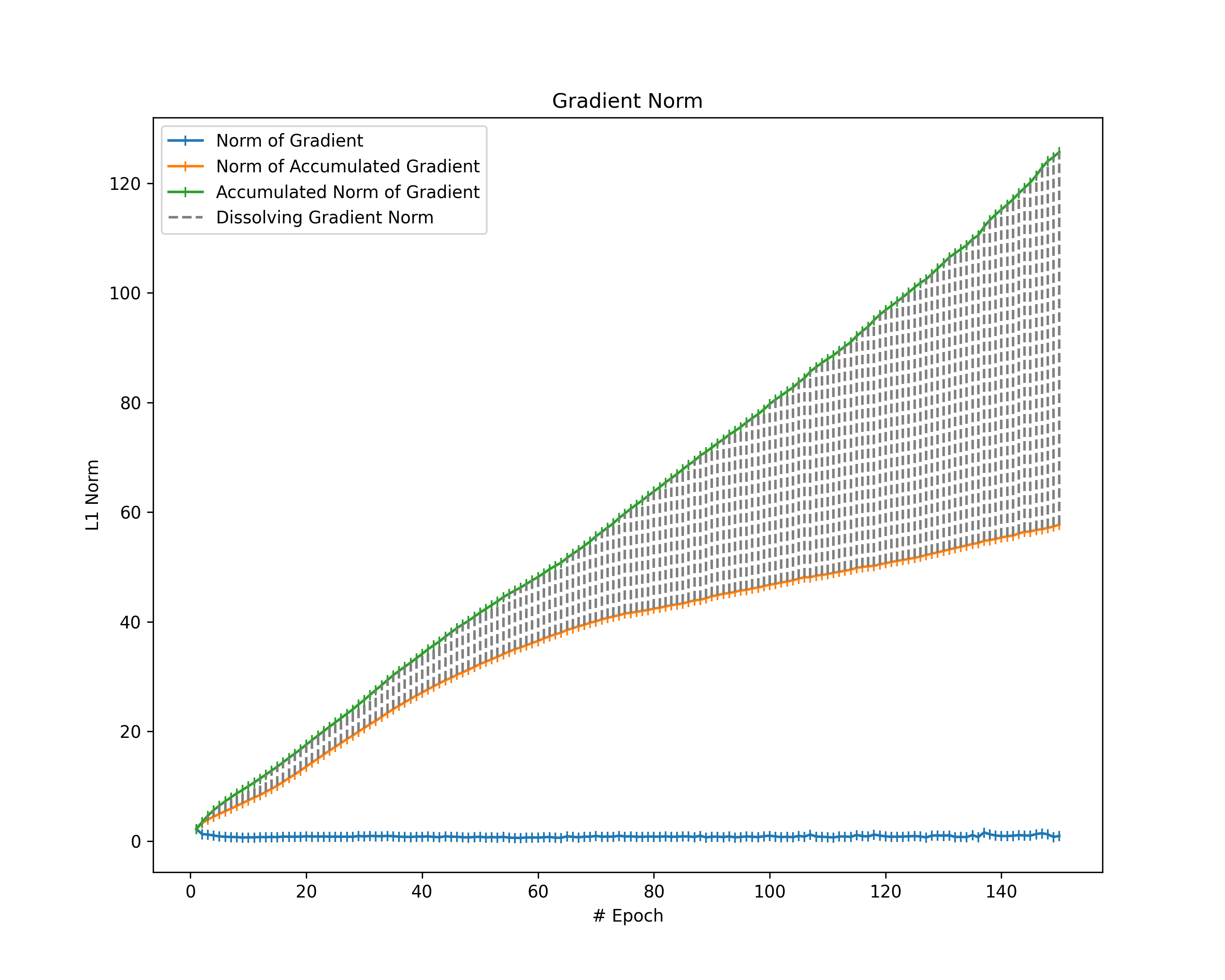
Note that the norm of the accumulated gradient is not necessarily the same as the accumulation of the gradient norms $$||\text{cumsum}(G)||_1 \leq \text{cumsum}(||G||_1)$$. This is because gradient elements usually do not keep the same direction throughout the whole training process and, hence, might dissolve themselves over the epochs (e.g., when zig-zagging). For that reason, we additionally compute the difference between the accumulation of gradient norms (i.e., the cumulative sum of the gradient norms) and the norm of the accumulated gradient to gather an idea of how much the gradients dissolve themselves during training. We call the resulting difference in norms “dissolving gradient norm”.

statistics["acc_l1_norm_standardized"] = np.cumsum(statistics["l1_norm_standardized"])
statistics["l1_dissolving_norm_standardized"] = statistics["acc_l1_norm_standardized"] - statistics["l1_norm_acc_standardized"]

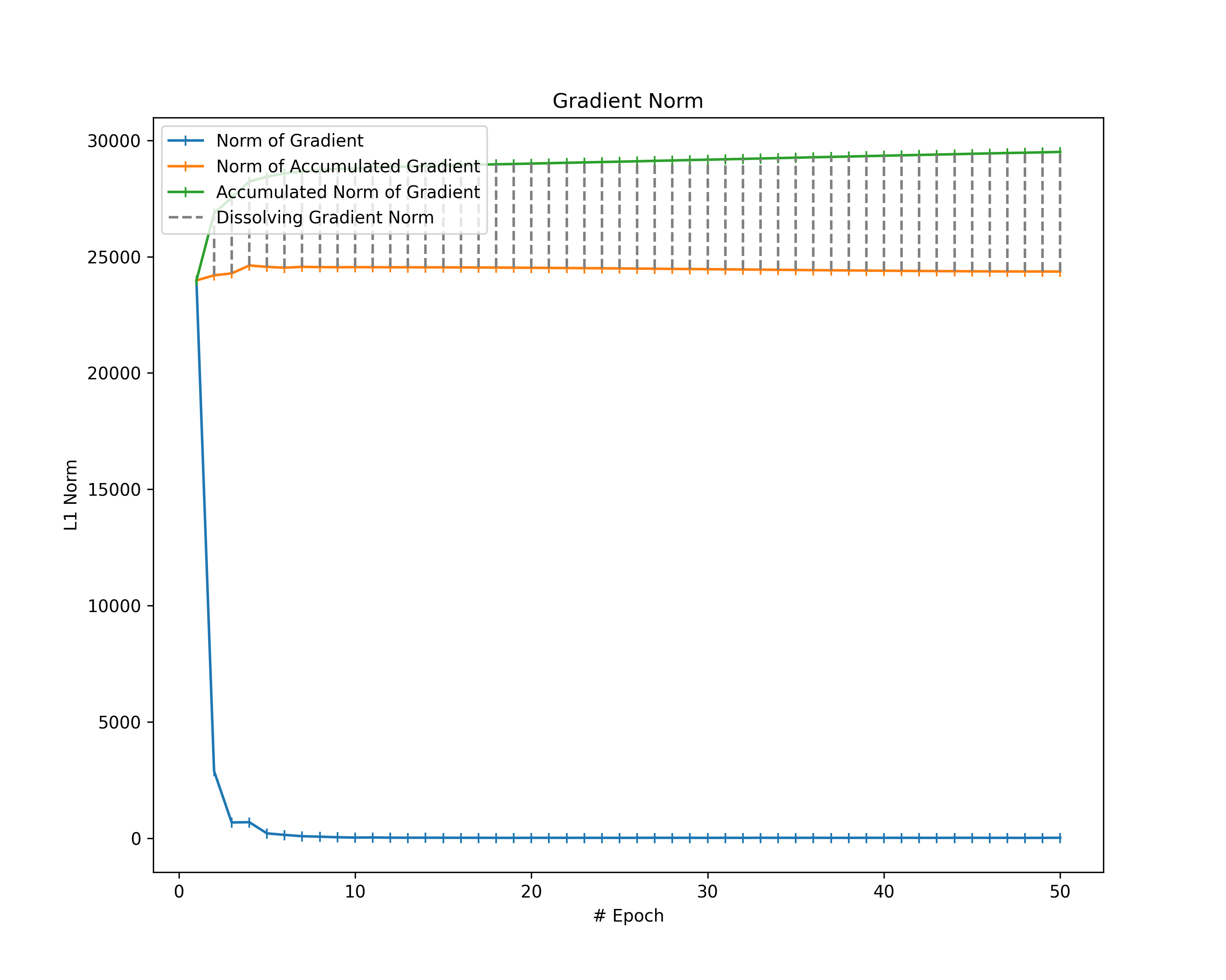
Finally, we plot all the gradient norms.

NUM_EPOCHS = len(gradients)
plt.figure(figsize=(10, 8), dpi=300)
plt.plot(range(1, NUM_EPOCHS+1), statistics["l1_norm_standardized"],
    linestyle="-", marker="|", label="Norm of Gradient")
plt.plot(range(1, NUM_EPOCHS+1), statistics["l1_norm_acc_standardized"],
    linestyle="-", marker="|", label="Norm of Accumulated Gradient")
plt.plot(range(1, NUM_EPOCHS+1), statistics["acc_l1_norm_standardized"],
    linestyle="-", marker="|", label="Accumulated Norm of Gradient")
plt.vlines(range(1, NUM_EPOCHS+1), statistics["l1_norm_acc_standardized"], statistics["acc_l1_norm_standardized"],
    linestyle="dashed", color="gray", label="Dissolving Gradient Norm")
plt.title("Gradient Norm")
plt.xlabel("# Epoch")
if(NUM_EPOCHS <= 20):
    plt.xticks(np.arange(1, NUM_EPOCHS+1, 1))
plt.ylabel("L1 Norm")
plt.legend(loc="upper left")
plt.savefig(figures_dir/r'gradient_norms.png')

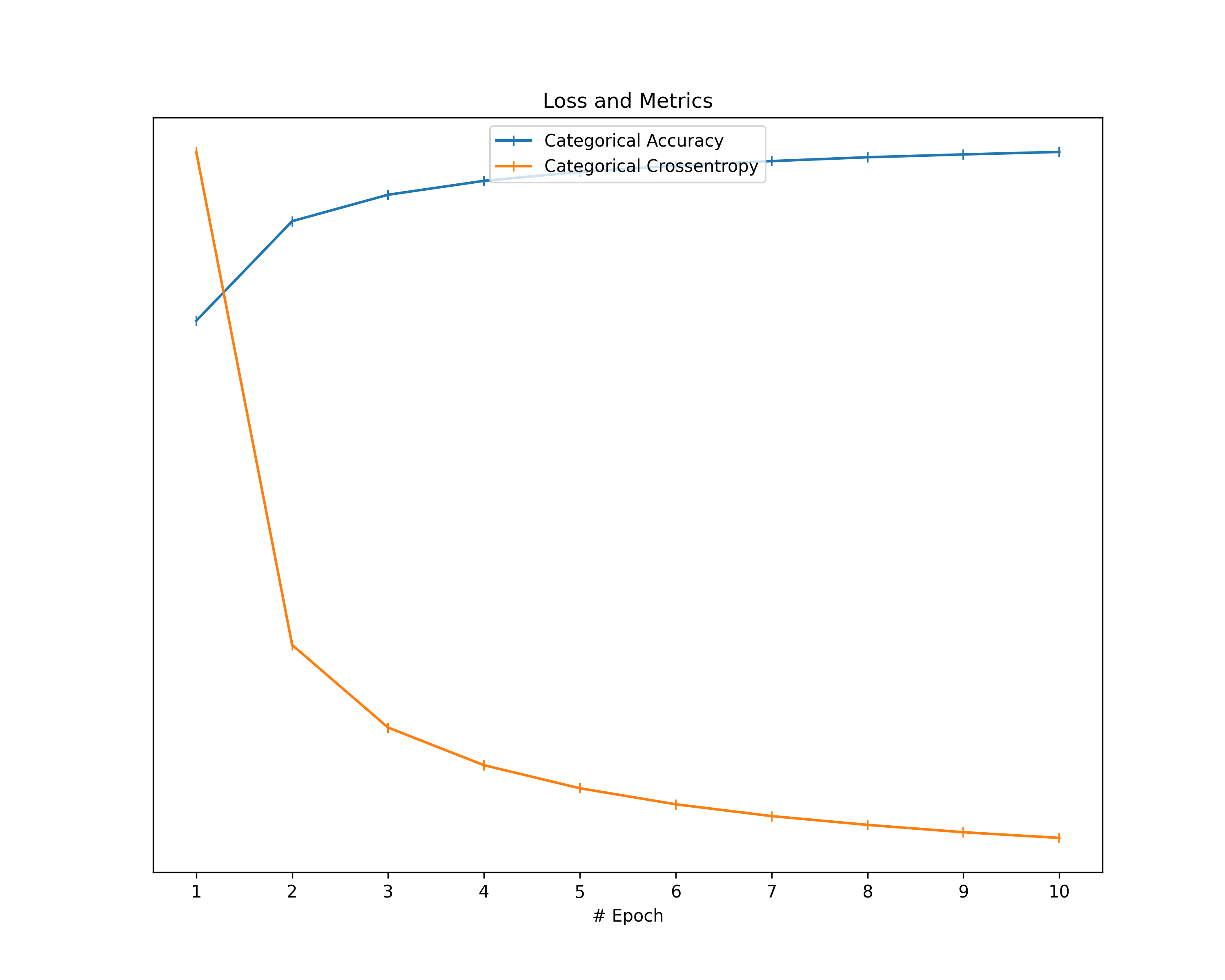
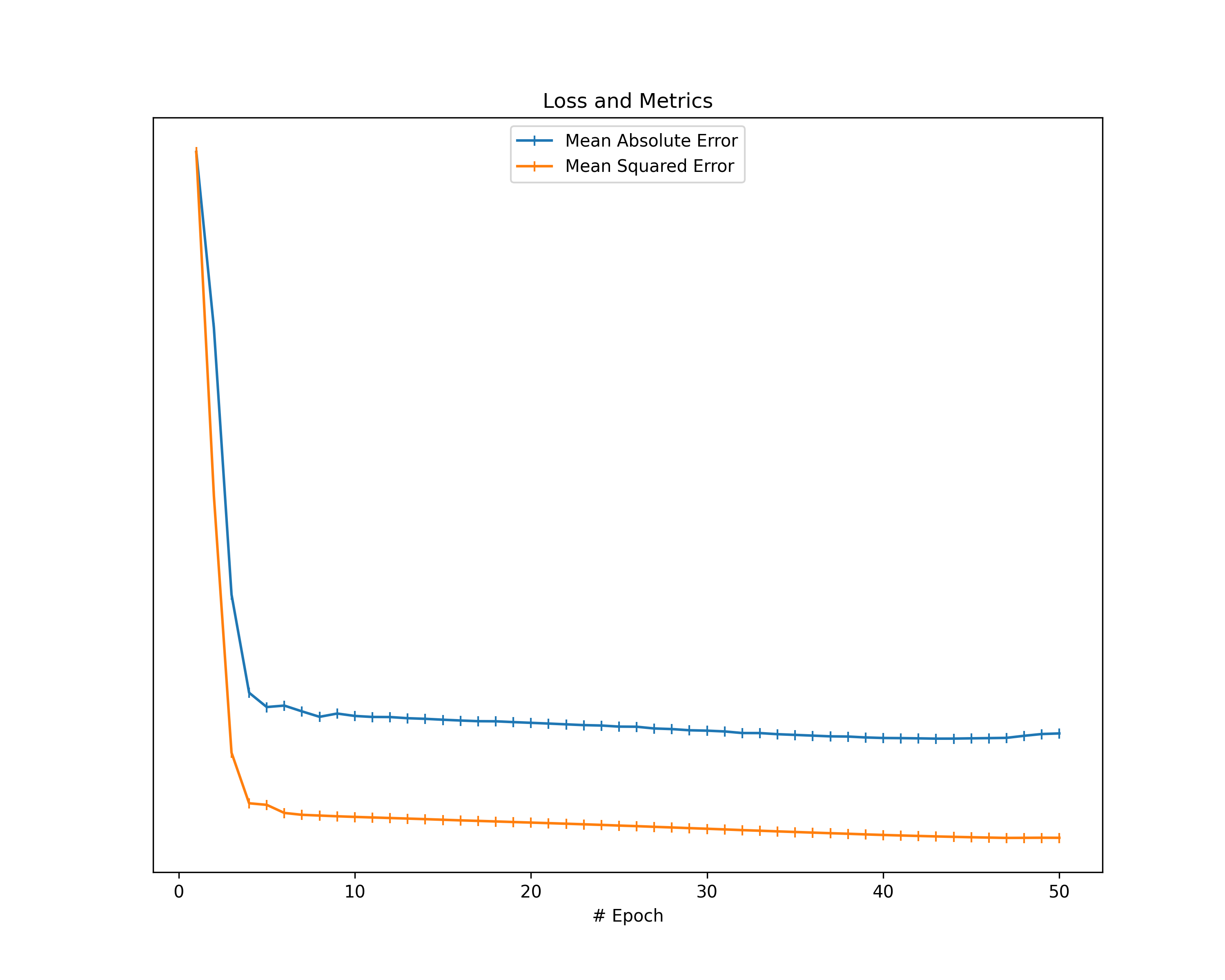
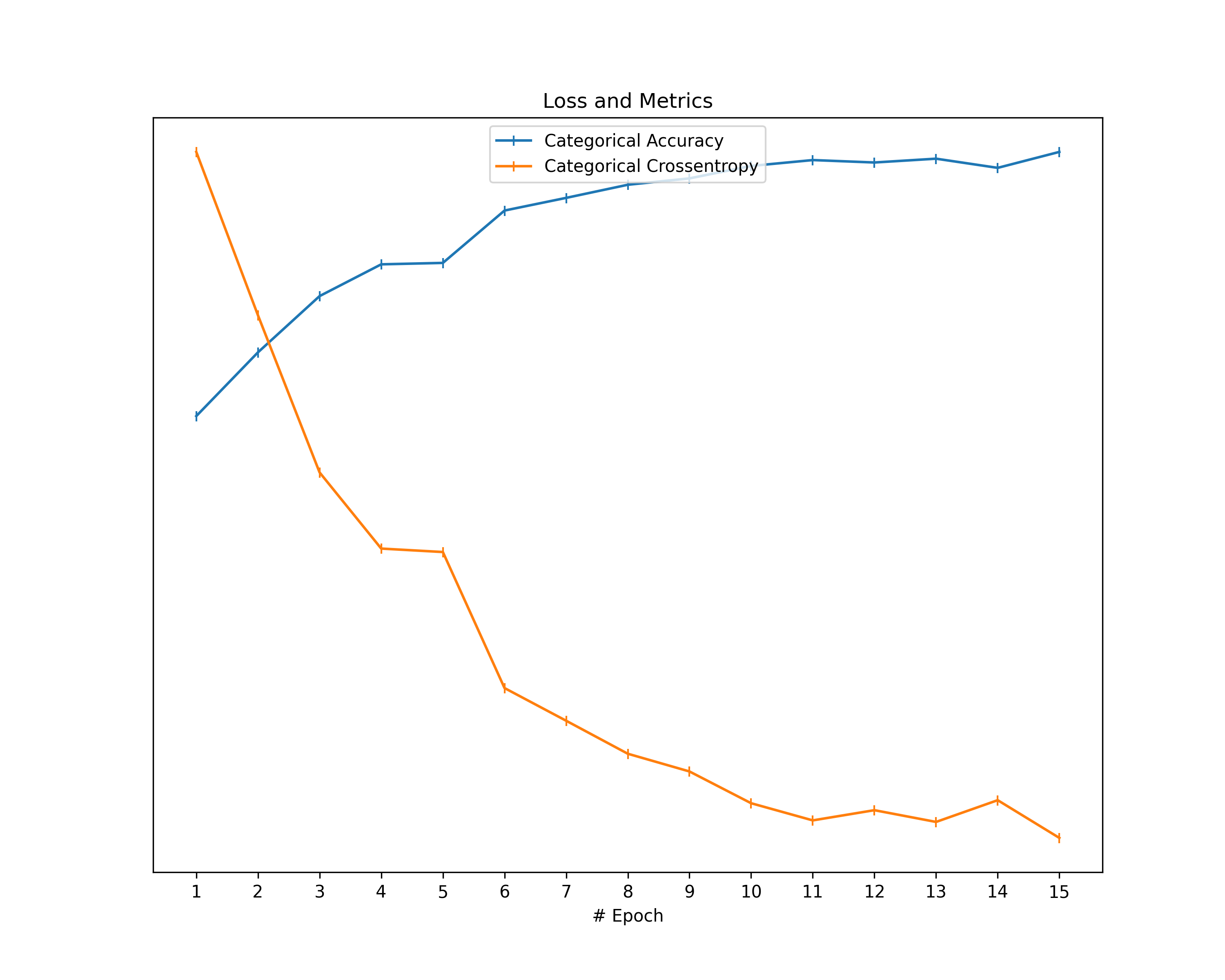
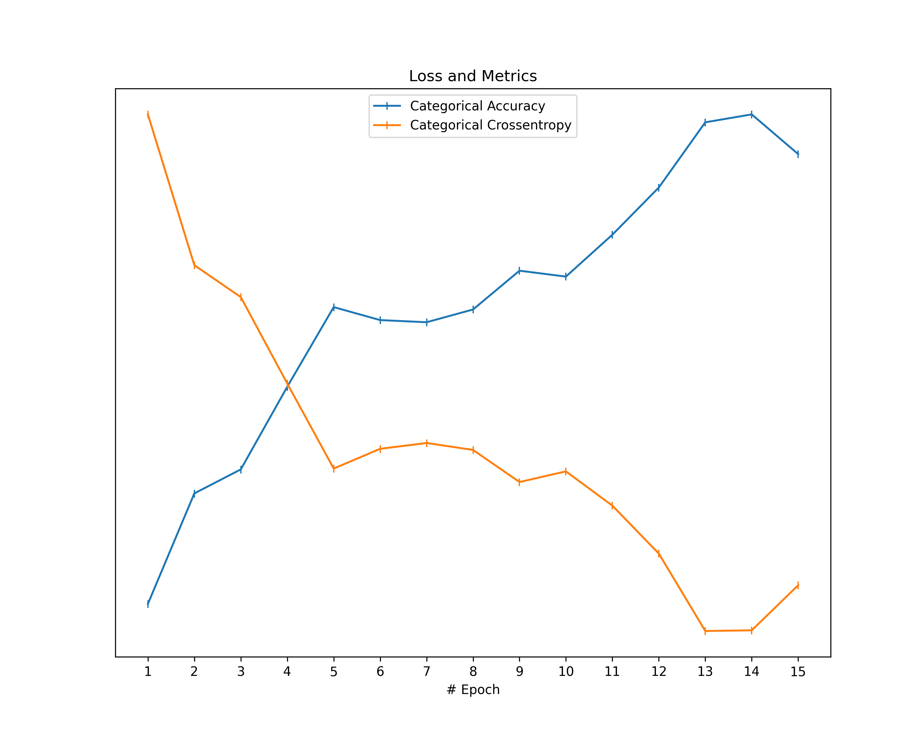
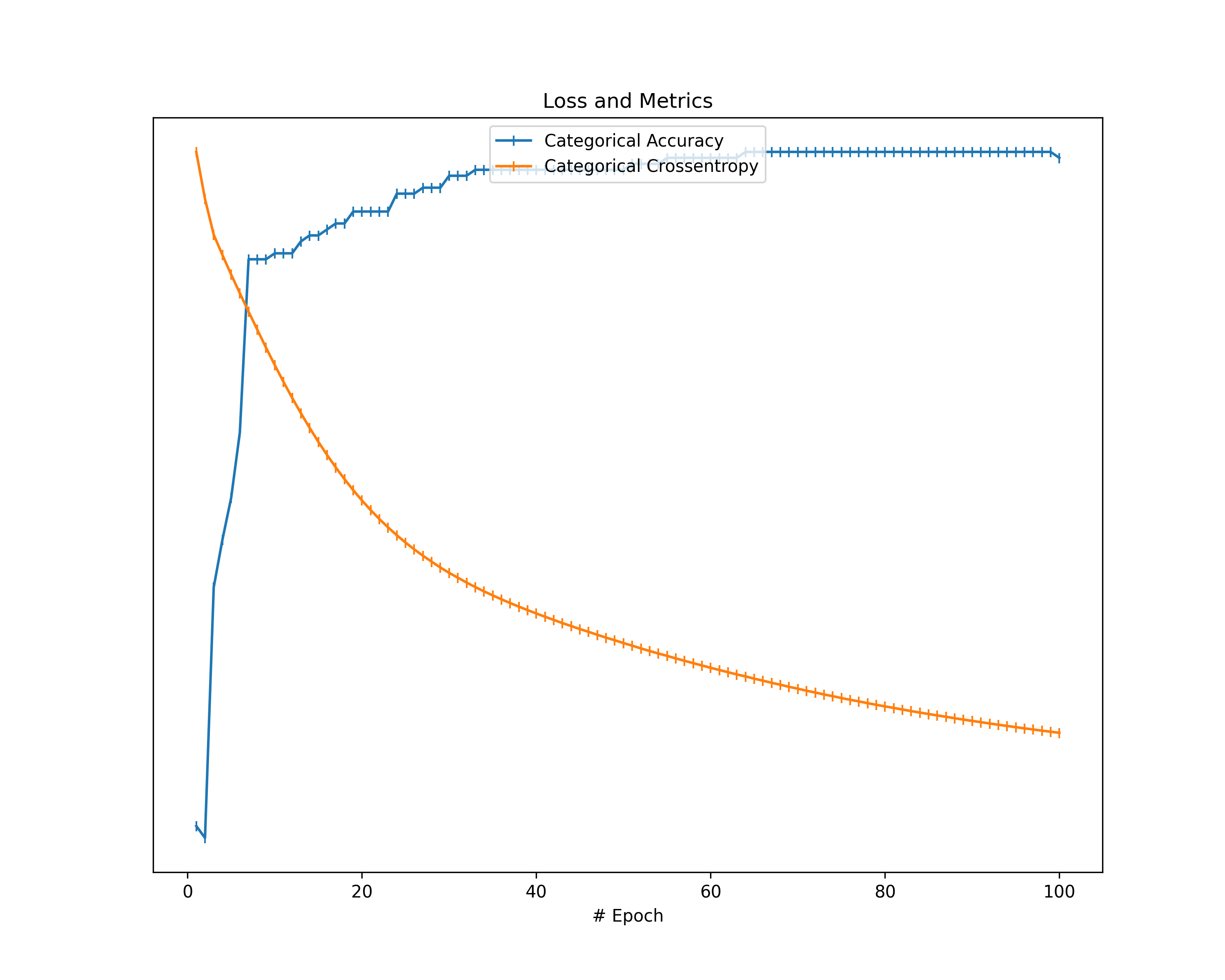
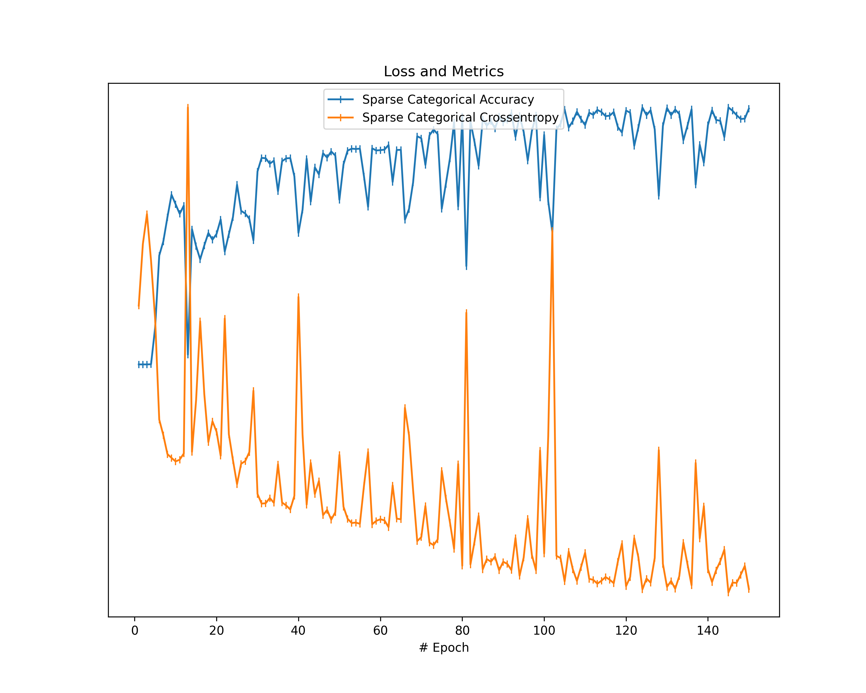
Of course, we also take the loss value as well as an additional metric into account and show them in a separate graph.

statistics["metrics"] = {metr_name: [metr[metr_name] for metr in metrics] for metr_name in metrics[0].keys()}
statistics["metrics"].pop('loss')

def scaleToMax1(arr):
    return np.array(arr) / np.max(np.array(arr))

plt.figure(figsize=(10, 8), dpi=300)
for metr_name, metr_arr in statistics["metrics"].items():
    plt.plot(range(1, NUM_EPOCHS+1), scaleToMax1(metr_arr), linestyle="-", marker="|", label=metr_name)
plt.title("Loss and Metrics")
plt.xlabel("# Epoch")
if(NUM_EPOCHS <= 20):
    plt.xticks(np.arange(1, NUM_EPOCHS+1, 1))
ax = plt.gca()
ax.get_yaxis().set_visible(False)
plt.legend(loc="upper center")
plt.savefig(figures_dir/r'loss.png')

Highest Gradient Value

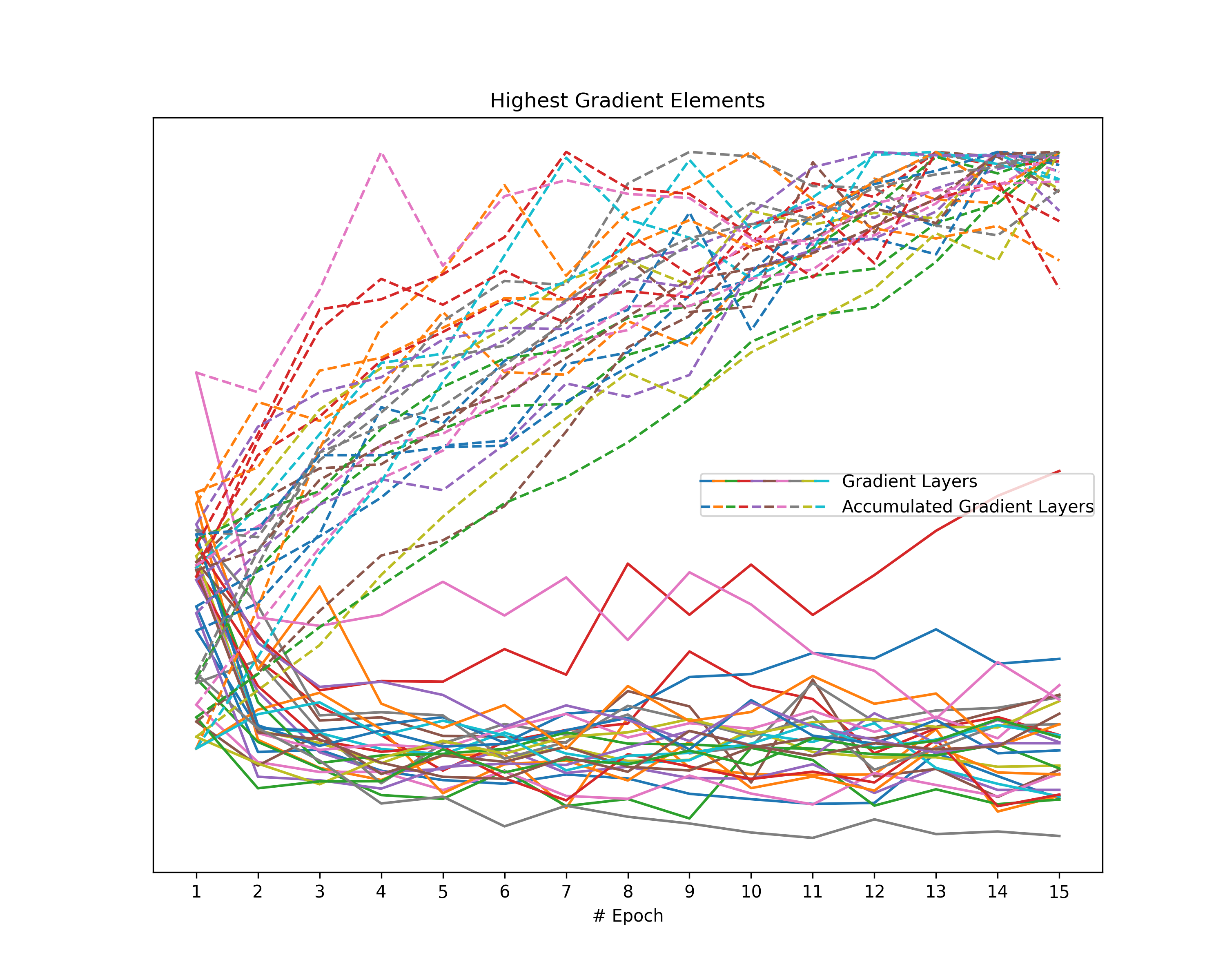
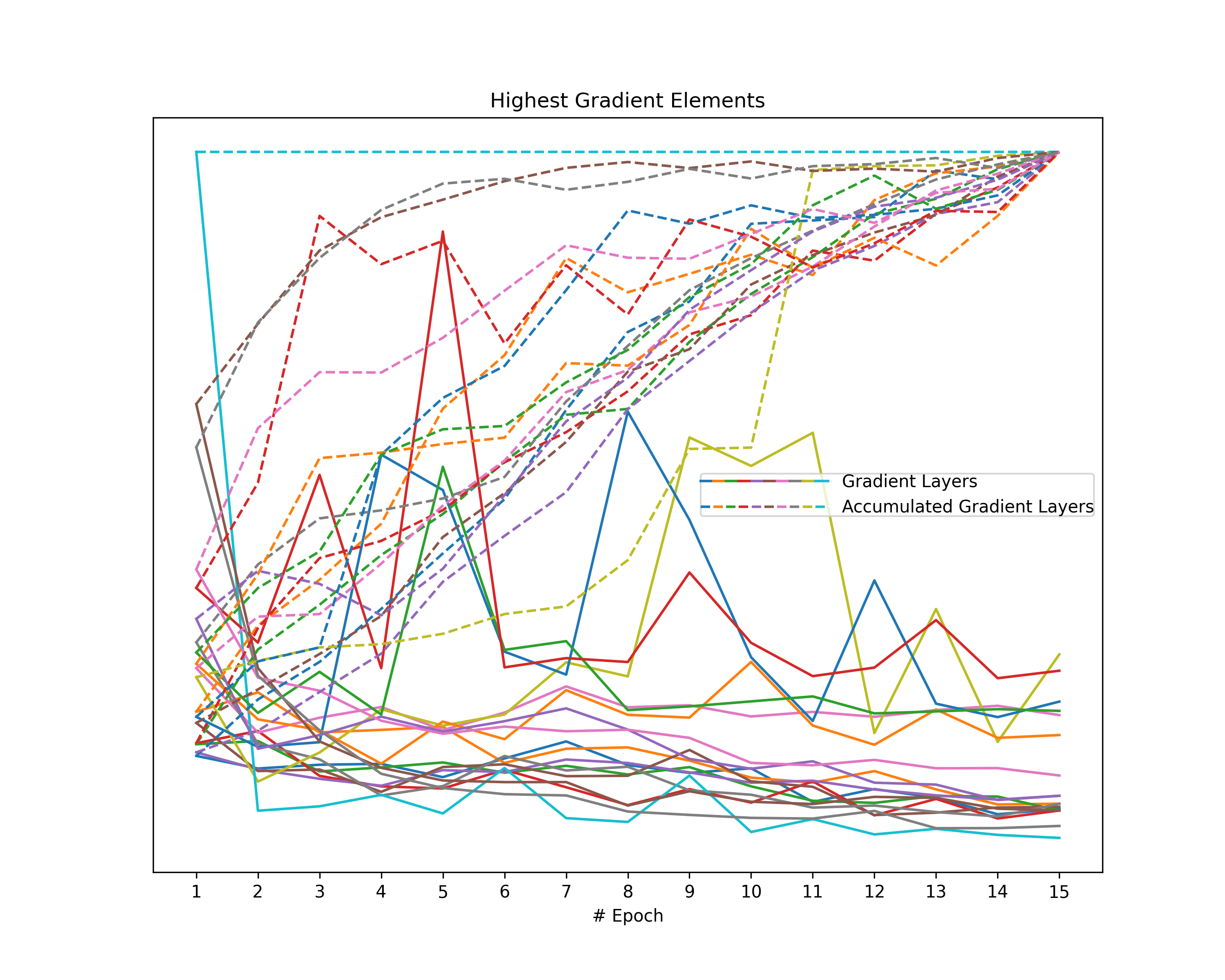
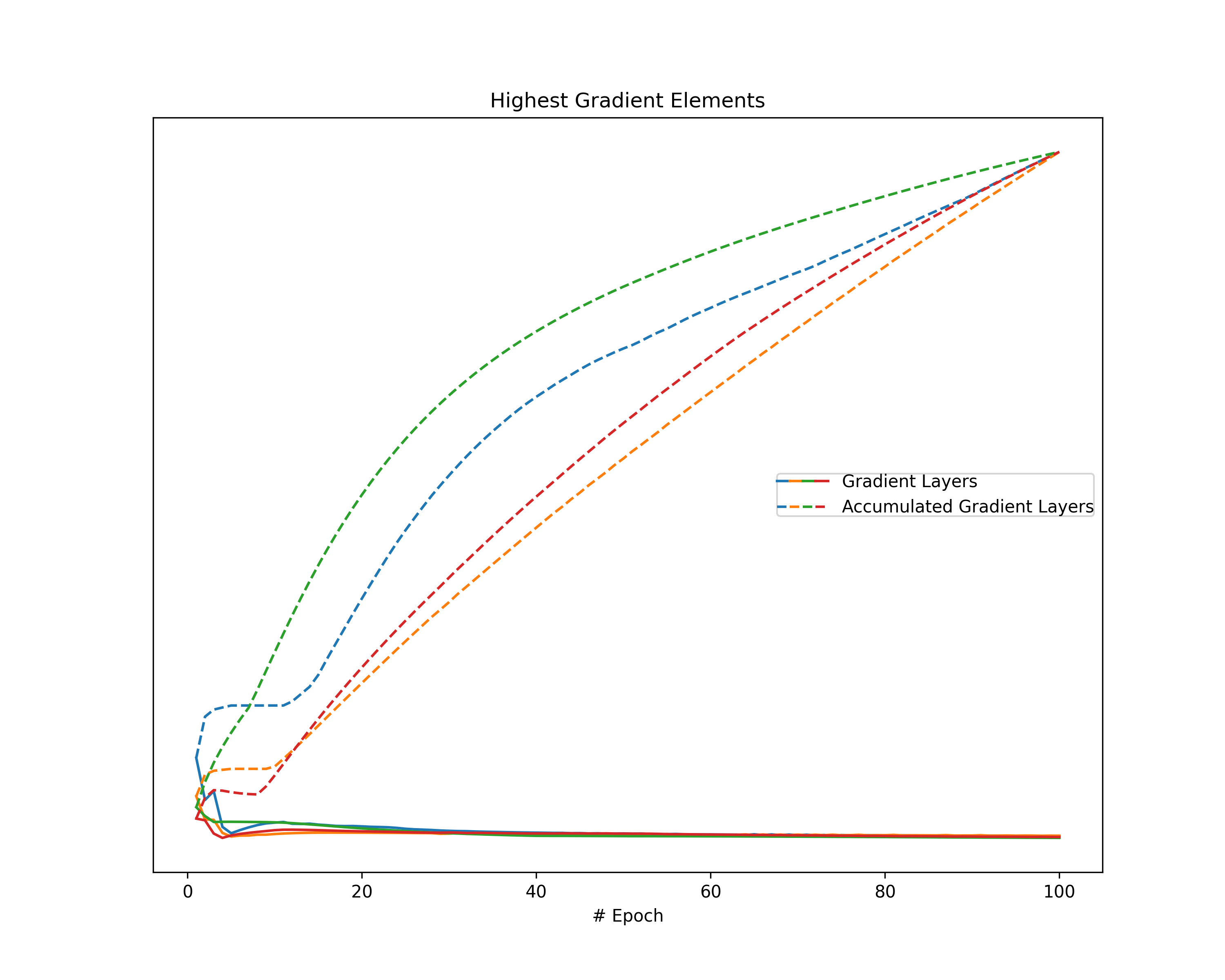
Another metric reflecting the magnitude of gradients is given by the highest value of a gradient. Since gradients describe both the direction and the strength of the optimization step, the highest absolute value indicates the gradient magnitude even though other values are extremely small (e.g., stress in a single dimension). However, since we cannot compare values across gradient layers of a neural network, we consider the highest layer-wise value. Note that, in an arbitrary neural network, not even values within the same layer are comparable. For that purpose, we assume fully connected layers.

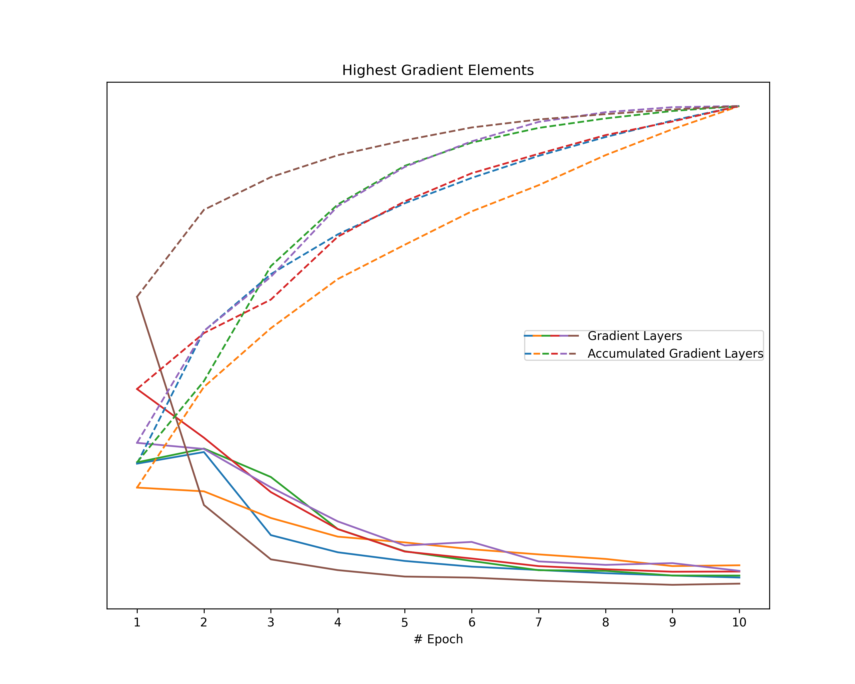
We obtain the highest element per gradient layer for each gradient as well as for each accumulated gradient. Note that we apply a layer-wise scaling to the gradient layer and the respective accumulated gradient over all epochs so that the highest values show a maximum of one.

accgrad_layer_scaling = [np.max(np.absolute(np.array(layer_grads).flatten()))
    for layer_grads in zip(*accumulated_gradients)]
accgrad_layer_scaling = [als if als != 0 else 1 for als in accgrad_layer_scaling]
accgrad_scaling = np.max(np.array(accgrad_layer_scaling))

grad_layer_highest_elements = [[np.max(np.absolute(layer_grad.flatten())) / accgrad_layer_scaling[counter]
        for counter, layer_grad in enumerate(grad)]
    for grad in gradients]
grad_highest_elements = np.max(np.array(grad_layer_highest_elements), axis=0)
grad_layer_highest_elements = np.array(list(zip(*grad_layer_highest_elements)))

accgrad_layer_highest_elements = [[np.max(np.absolute(layer_grad.flatten())) / accgrad_layer_scaling[counter]
        for counter, layer_grad in enumerate(accgrad)]
    for accgrad in accumulated_gradients]
accgrad_highest_elements = np.max(np.array(accgrad_layer_highest_elements), axis=0)
accgrad_layer_highest_elements = np.array(list(zip(*accgrad_layer_highest_elements)))

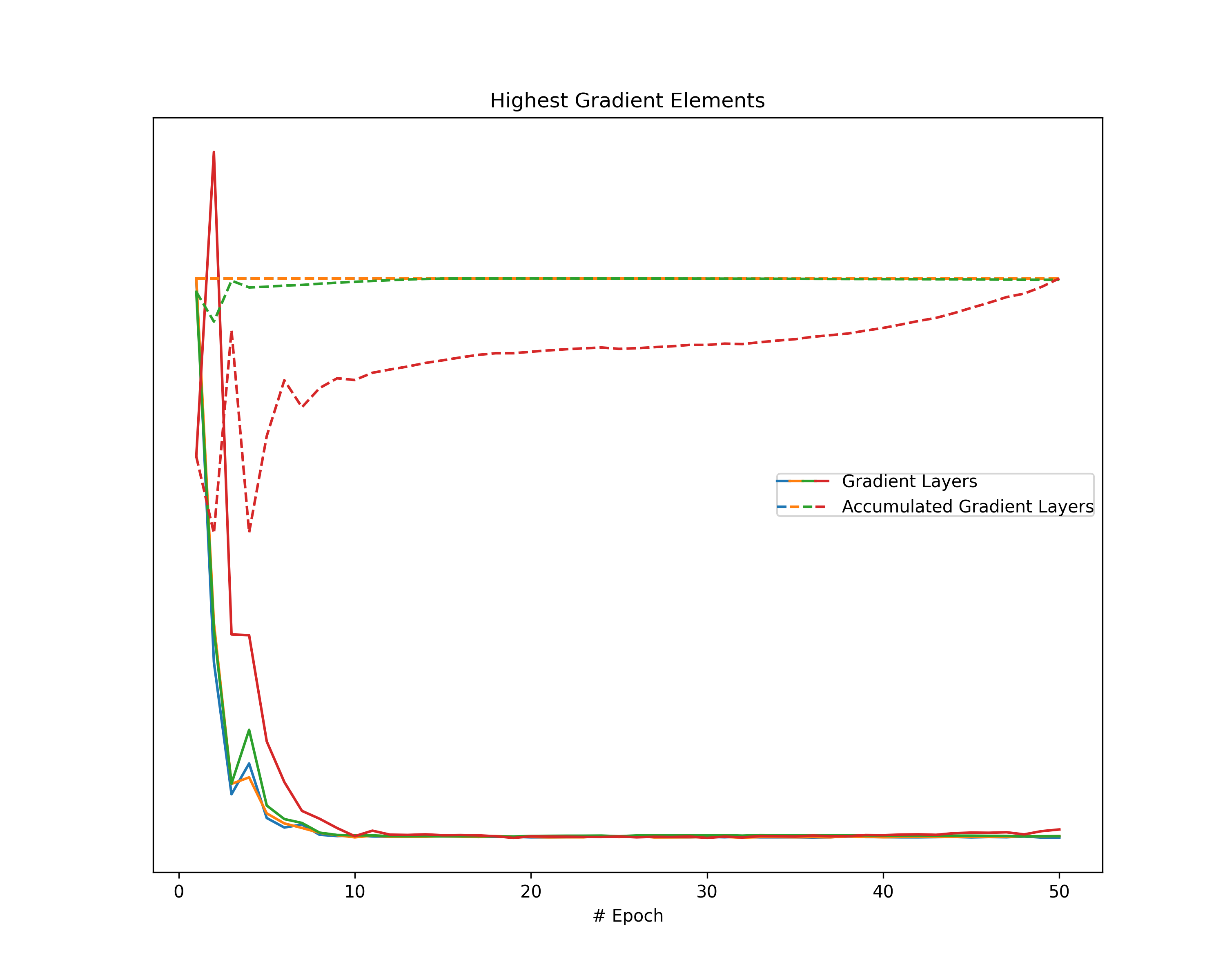
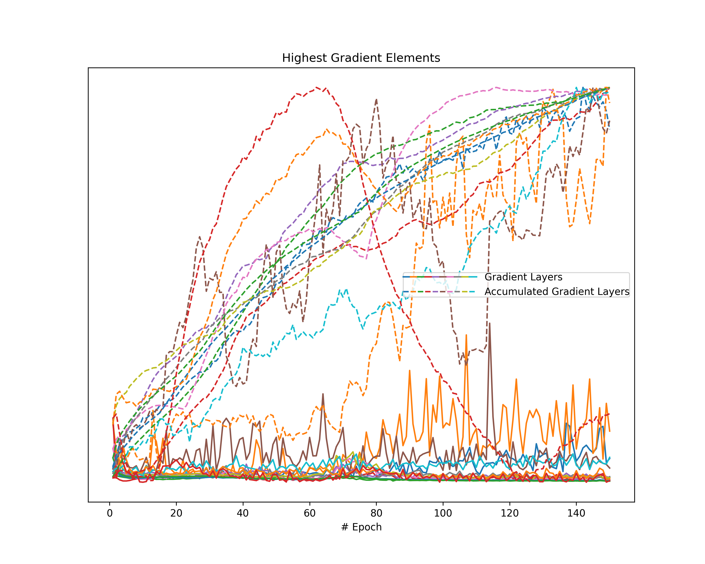
Having gathered these highest gradient values, we visualize them in a line plot.

plt.figure(figsize=(10, 8), dpi=300)
glhe_lines = list()
for counter, glhe in enumerate(grad_layer_highest_elements):
    glhe_lines.append(plt.plot(range(1, NUM_EPOCHS+1), glhe, color=f'C{counter}',
        label=f'Grad Layer {counter}')[0])
alhe_lines = list()
for counter, alhe in enumerate(accgrad_layer_highest_elements):
    alhe_lines.append(plt.plot(range(1, NUM_EPOCHS+1), alhe, color=f'C{counter}',
        linestyle='dashed', label=f'Accgrad Layer {counter}')[0])

glhe_lines = glhe_lines[:10]
alhe_lines = alhe_lines[:10]

plt.title("Highest Gradient Elements")
plt.xlabel("# Epoch")
if(NUM_EPOCHS <= 20):
    plt.xticks(np.arange(1, NUM_EPOCHS+1, 1))
ax = plt.gca()
ax.get_yaxis().set_visible(False)
plt.legend([tuple(glhe_lines), tuple(alhe_lines)], ["Gradient Layers", "Accumulated Gradient Layers"],
    numpoints=1, handler_map={tuple: HandlerTuple(ndivide=None)}, borderpad=0,
    handlelength=len(glhe_lines)*0.75, loc="center right")
plt.savefig(figures_dir/r'highestgradelement.png')

Animation

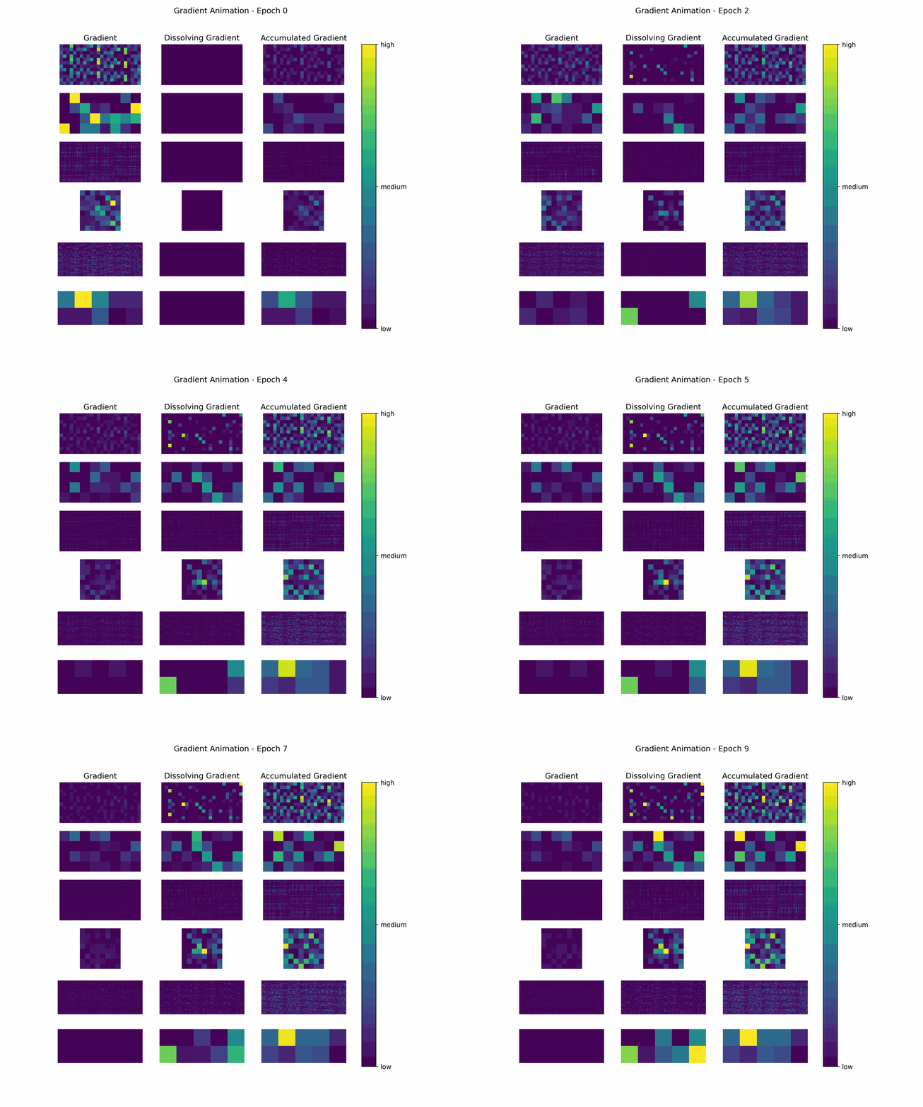
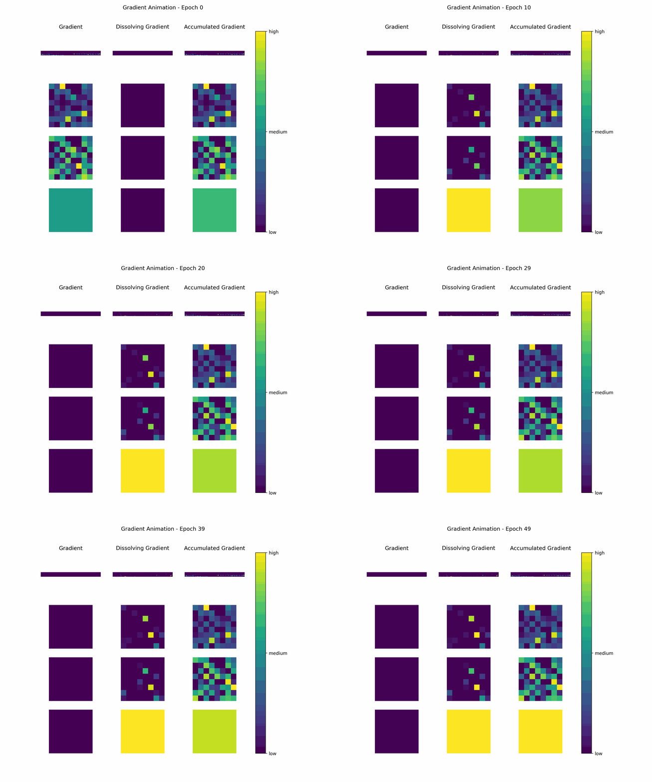
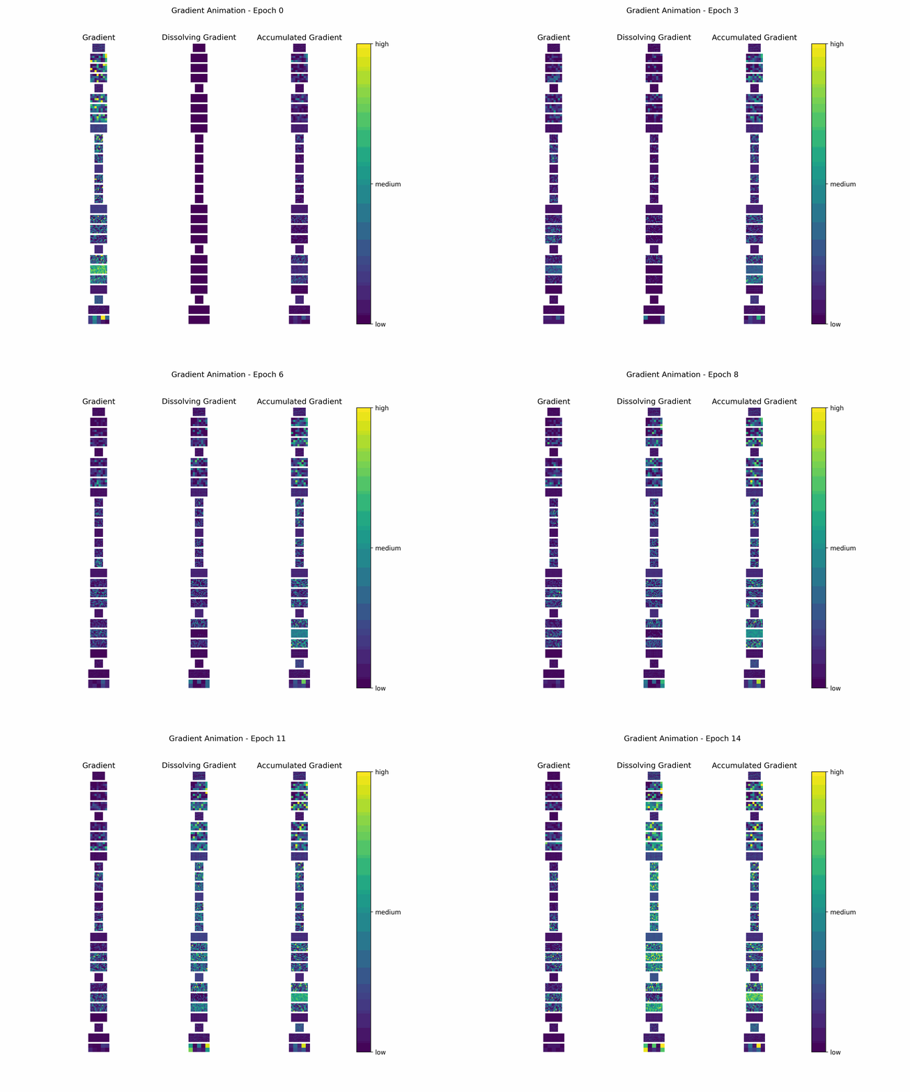
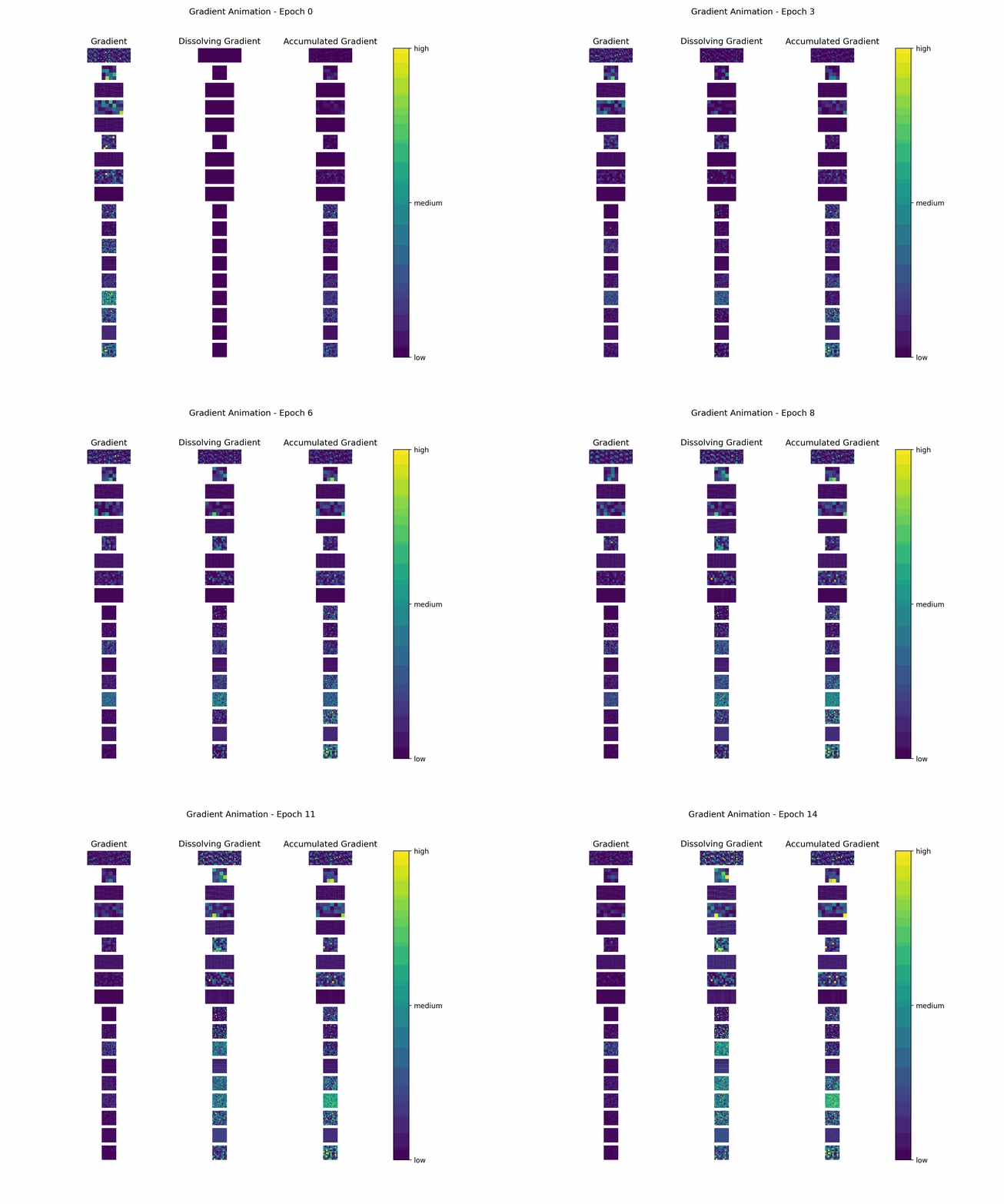
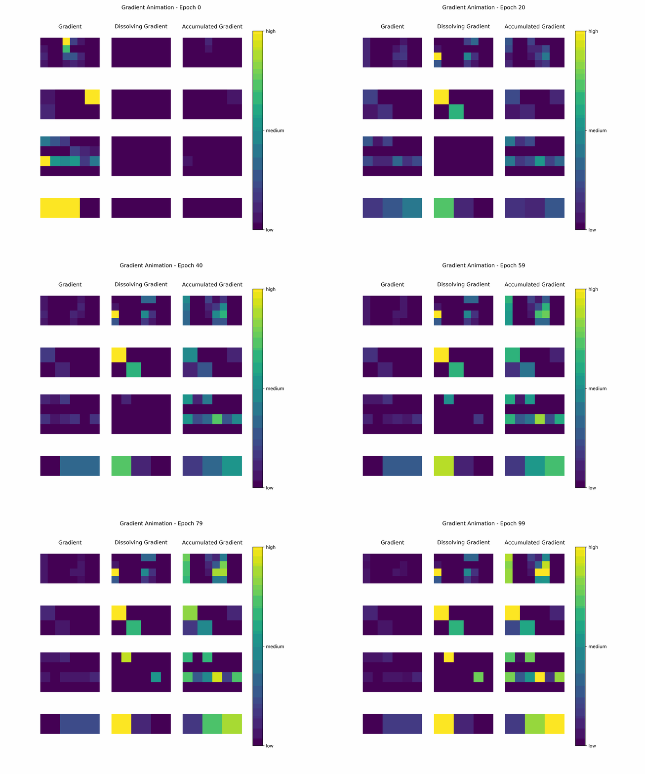
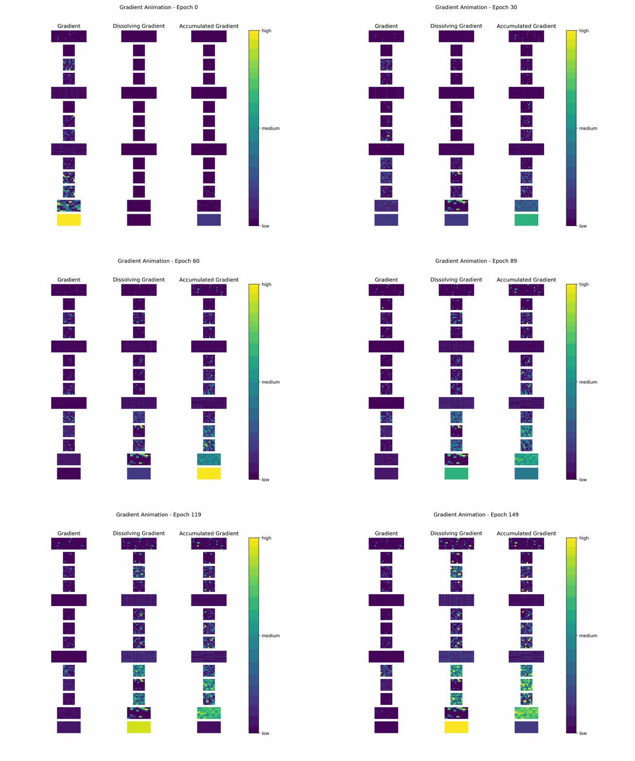
In order to gain further insight into the behavior of a gradient during training — with the main focus on its magnitude —, we create animations showing heatmaps of our gradient layers. Thereby, we can visually obtain the impact of the gradient layers at a specific training epoch. We perform this for the gradients and the accumulated gradients so that we can compare the gradient’s magnitude to its respective impact on the model. Additionally to these gradients, we compute the difference between the accumulation of absolute gradients and the accumulated gradient to provide insights on dissolving gradient elements. Dissolving gradient elements are values of a gradient that are equalized in the accumulated gradient by a successive gradient.

accumulated_absolute_gradients = np.cumsum(np.absolute(gradients), axis=0)
dissolving_gradients = accumulated_absolute_gradients - np.absolute(accumulated_gradients)

Before creating the heatmaps, we scale each layer by the highest absolute value of the respective layer over all epochs.

grad_layer_scaling = [np.max(np.absolute(np.array(layer_grads).flatten()))
    for layer_grads in zip(*gradients)]
grad_layer_scaling = [gls if gls != 0 else 1 for gls in grad_layer_scaling]
grad_scaling = np.max(np.array(grad_layer_scaling))

dissgrad_layer_scaling = [np.max(np.absolute(np.array(layer_grads).flatten()))
    for layer_grads in zip(*dissolving_gradients)]
dissgrad_layer_scaling = [dls if dls != 0 else 1 for dls in dissgrad_layer_scaling]
dissgrad_scaling = np.max(np.array(dissgrad_layer_scaling))

accgrad_layer_scaling = [np.max(np.absolute(np.array(layer_grads).flatten()))
    for layer_grads in zip(*accumulated_gradients)]
accgrad_layer_scaling = [als if als != 0 else 1 for als in accgrad_layer_scaling]
accgrad_scaling = np.max(np.array(accgrad_layer_scaling))

Then, we create an animation plot using Matplotlib that shows layer-wise heatmaps for the gradients, the accumulated gradients, and the dissolved gradient elements. Note that the heatmap shapes are an arbitrarily chosen matrix to visualize the individual layers better. Also note that we scale every gradient type (i.e., gradient, accumulated gradient, dissolved gradient) independently to a range from 0 to 1, and, hence, we cannot utilize these heatmaps to compare values among gradient types.

# Function to obtain the prime factors for gradient layer reshaping
def prime_factors(n):
    i = 2
    factors = []
    while i * i <= n:
        if n % i:
            i += 1
        else:
            n //= i
            factors.append(i)
    if n > 1:
        factors.append(n)
    return factors

# Plot heatmap animation of gradients
fig = plt.figure(figsize=(10, 8), dpi=300)
fig_gridspec = fig.add_gridspec(1, 3)

# Gradients
grad_gridspec = fig_gridspec[0, 0].subgridspec(len(gradients[0]), 1)
ax_grad = fig.add_subplot(grad_gridspec[:, 0])
ax_grad.axis("off")
ax_grad.set_title("Gradient")

def showGrad(i):
    for counter, layer_grad in enumerate(gradients[i]):
        primfac = prime_factors(layer_grad.size)
        p = int(np.prod([elem for idx, elem in enumerate(primfac) if idx % 2 == 0]))
        q = int(np.prod([elem for idx, elem in enumerate(primfac) if idx % 2 == 1]))
        ax = fig.add_subplot(grad_gridspec[counter, 0])
        # layer-wise scaling between 0 and 1
        ax.imshow(np.absolute(layer_grad.reshape((min(p, q), max(p, q))) / grad_layer_scaling[counter]), vmin=0, vmax=1)
        ax.set_axis_off()

# Dissolving Gradients
dissgrad_gridspec = fig_gridspec[0, 1].subgridspec(len(dissolving_gradients[0]), 1)
ax_dissgrad = fig.add_subplot(dissgrad_gridspec[:, 0])
ax_dissgrad.axis("off")
ax_dissgrad.set_title("Dissolving Gradient")

def showDissGrad(i):
    for counter, layer_grad in enumerate(dissolving_gradients[i]):
        primfac = prime_factors(layer_grad.size)
        p = int(np.prod([elem for idx, elem in enumerate(primfac) if idx % 2 == 0]))
        q = int(np.prod([elem for idx, elem in enumerate(primfac) if idx % 2 == 1]))
        ax = fig.add_subplot(dissgrad_gridspec[counter, 0])
        # layer-wise scaling of gradient between 0 and 1
        ax.imshow(np.absolute(layer_grad.reshape((min(p, q), max(p, q))) / dissgrad_layer_scaling[counter]), vmin=0, vmax=1)
        ax.set_axis_off()

# Accumulated Gradients
accgrad_gridspec = fig_gridspec[0, 2].subgridspec(len(accumulated_gradients[0]), 1)
ax_accgrad = fig.add_subplot(accgrad_gridspec[:, 0])
ax_accgrad.axis("off")
ax_accgrad.set_title("Accumulated Gradient")

def showAccGrad(i):
    for counter, layer_grad in enumerate(accumulated_gradients[i]):
        primfac = prime_factors(layer_grad.size)
        p = int(np.prod([elem for idx, elem in enumerate(primfac) if idx % 2 == 0]))
        q = int(np.prod([elem for idx, elem in enumerate(primfac) if idx % 2 == 1]))
        ax = fig.add_subplot(accgrad_gridspec[counter, 0])
        # layer-wise scaling of gradient between 0 and 1
        ax.imshow(np.absolute(layer_grad.reshape((min(p, q), max(p, q))) / accgrad_layer_scaling[counter]), vmin=0, vmax=1)
        ax.set_axis_off()

def showGradients(i):
    fig.suptitle(f'Gradient Animation - Epoch {i}')
    showGrad(i)
    showDissGrad(i)
    showAccGrad(i)

# create colorbar
cbar = fig.colorbar(None, ax=fig.get_axes())
fig.subplots_adjust(right=0.75)
cbar.set_ticks([0, 0.5, 1])
cbar.set_ticklabels(['low', 'medium', 'high'])

anim = animplt.FuncAnimation(fig, showGradients, frames=NUM_EPOCHS, interval=1000)
anim.save(figures_dir/r'animation.gif', writer=animplt.PillowWriter(fps=1))

Evaluation

In this section, we present the results for all of our datasets and interpret the structures and shapes that appear in the plots. This way, we try to identify the general behavior of gradients during training.

The results consist of the following plots:

Training Loss: Shows the loss and an additional metric during training and gives a general confirmation about the correctness of training.
Gradient Norms: Reflects the magnitudes of the gradients and the magnitude of their respective accumulation accompanied by an indication of how much of the gradient has been dissolved by reverting elements during training.
Highest Gradient Elements: Displays the behavior of the highest elements inside gradient layers during training.
Gradient Animation: Shows the magnitudes of gradient elements in a heatmap.

Mnist

Boston Housing

Highest Gradient Elements - Boston Housing

Cifar10

Cifar100

Iris

FordA

Interpretation

Training Loss: The plots about the training loss and an additional metric show a decrease in loss and an improvement in the respective metric for all our datasets. This behavior confirms the correctness of our models in terms of learning from the data provided.

Gradient Norms: When looking at the norm of our gradients and considering them as the magnitudes of the gradients, we observe a decrease in gradient magnitude over the epochs in most of the plots. Furthermore, all plots show that the norm of the accumulated gradients does not follow a linear relationship with the epochs. There are two potential sources for such a non-linear behavior: Either the magnitude of our gradients decreases (as already observed) or the gradients partially dissolve themselves during training. To identify the extent of dissolving gradient elements, we look at the distance between the norm of accumulated gradients and the accumulated gradient norms. Thereby, we can also determine whether the magnitude of our gradients decreases over time. If the accumulated norms of our gradients follow a straight line, the magnitude of the individual gradients is constant. The opposite behavior (accumulated norms of gradients following a curve) indicates a decrease of the magnitude.

Highest Gradient Elements: Investigation on the layer-wise highest element of both the gradients and the accumulated gradients indicates a common behavior in all plots. The magnitude of our gradients mainly decreases over the epochs, while the magnitude of the accumulated gradient increases. Therefore, we observe a clear separation of the respective lines in our plots, despite a single layer of the accumulated gradient in the case of the FordA model.

Gradient Animation: The layer-wise heatmap-animations of the gradients show high values at the very beginning of the training processes. Hand in hand, the accumulated gradients show a strong increase due to the accumulation of these very high gradients. Also, our dissolving gradient experiences a stronger gain in the early epochs. However, all these gradients seem almost constant as the epochs evolve. Altogether, the behavior of decreasing gradients while the accumulated gradients increase indicates a general reduction in the magnitude of gradients during the learning process.

Conclusion

Based on the above results, we can conclude that the accumulated gradients become weaker the more our model learns. Another interesting fact is that either the gradients decrease over the epochs or our dissolving gradient increases. Since an increase in the magnitude of dissolving gradients indicates that we are not actually learning, we can also conclude that the gradients diminish as our model approaches an optimum.

Acknowledgments

This work has been conducted during my employment at Know Center Research GmbH within the Pro’k’ress project funded by FFG.